
Using Elasticsearch and Kibana for Garbage Collection Log Analysis
jtendo provides a wide variety of telco software, and yes, some of these systems are written in Java. All these systems have to follow industry standards providing service with highest possible speed and 99.999 availability.
As you probably know, Java uses garbage collection and this may cause some performance issues if not tuned properly. For example, if garbage collector stops application threads for too long it may disrupt request processing or cause a cluster node restart. Therefore, it is very important to monitor garbage collection process and tune JVM settings to avoid problems and achieve highest possible capacity with minimal GC impact.There are several tools for GC analysis available and all come with some pros and cons. Since we advocate usage of Elasticsearch among our customers I’ve decided to implement my own tool based on Elasticsearch with graphs crafted in Kibana and some simple script to parse and index data.
How to monitor GC?
There are several tools that allow monitoring of JVM memory in both plain text and graphical mode. Some of those tools come bundled with JDK (jstat, jconsole) while other have to be installed separately (visualvm).
What if jstat gives too little information and you cannot use neither jconsole nor visualvm due to e.g. concerns about performance impact? There is another option – GC logs. This feature is very easy to use and comes bundled with most modern-day java distributions. JVM simply logs various information about progress and outcome of garbage collection process to a plain text file in human readable form. If you’re concerned about disk resources – there are options which allow control of verbosity and log rotation limiting disk footprint.
GC log example
As said – gc logs come in human readable format. But what exactly is logged to such a file? Here is an excerpt from one G1 GC event logged by telecom application server1:
[2024-11-13T11:37:15.968+0100][11624728.830s][info ][gc,start ] GC(437999) Pause Young (Mixed) (G1 Evacuation Pause)
[2024-11-13T11:37:16.179+0100][11624729.041s][info ][gc,heap ] GC(437999) Eden regions: 166->0(191)
[2024-11-13T11:37:16.179+0100][11624729.041s][info ][gc,heap ] GC(437999) Survivor regions: 32->7(25)
[2024-11-13T11:37:16.179+0100][11624729.041s][info ][gc,heap ] GC(437999) Old regions: 1813->1732
[2024-11-13T11:37:16.179+0100][11624729.041s][info ][gc,heap ] GC(437999) Humongous regions: 13->13
[2024-11-13T11:37:16.179+0100][11624729.041s][info ][gc,metaspace ] GC(437999) Metaspace: 179449K->179449K(1222656K)
[2024-11-13T11:37:16.179+0100][11624729.041s][info ][gc ] GC(437999) Pause Young (Mixed) (G1 Evacuation Pause) 16181M->14004M(31744M) 210.828ms
[2024-11-13T11:37:16.179+0100][11624729.041s][info ][gc,cpu ] GC(437999) User=8.25s Sys=0.41s Real=0.21s
We have several lines from GC event number 437999. This is a mixed GC cycle which means it will collect young generation along with a portion of regions from old. Following lines provide detailed information on heap changes due to objects relocation with indication how many regions were utilised by each type before and after GC.
At the end we have two lines which summarise both performance and result of this particular GC. We know that heap utilization was reduced from 16181MB to 14004 MB while total capacity is 31744MB and that application was paused for around 211ms. The last line contains information on CPU saying that all threads spent 8,25s in user mode and 0,41s in kernel mode while it took 0,21s of wall-clock time.
How to feed it to Elasticsearch?
To be able to utilize whole power of ELK stack first we have to index all that data. Using Filebeat and Logstash with some help of Grok patterns is one possible approach. What I decided to do instead is to write my own simple script that will do all the necessary parsing and indexing. There is a huge number of supported programming languages – you can always write the script in your favourite one2. As JSON is the format used by HTTP API of Elasticsearch the data presented above gets parsed (with a little help of regular expressions and capture groups) to a following JSON document:
{
„@timestamp”: „2024-11-13T11:37:16.179+0100”,
„gc_id”: 437999,
„gc_pause_type”: „G1 Evacuation Pause”,
„gc_type”: „Young (Mixed)”,
„time_since_start”: „11624729.041”,
„before”: { „eden_length”: 166, „heap”: 16181, „humongous_length”:
13, „metaspace”: 179449, „old_length”: 1813, „survivor_length”: 32 },
„after”: { „eden_length”: 0, „heap”: 14004, „humongous_length”:
13, "metaspace”: 179449, „metaspace_reserved”: 1222656, „old_length”:
1732, "survivor_length": 7 },
„cpu”: { „real”: 0.21, „sys”: 0.41, „user”: 8.25 },
"heap_max": 31744,
„pause_gc_duration”: 210.828
}
Once we have all the data in Elasticsearch we can start creating charts and dashboards. Even though the above example explains G1 GC log you can still use it for any garbage collector you have in your environment.

Examples
Memory leak
Sometimes memory leaks can be very tricky to find. Especially if it runs slowly for a long period of time. Watching saw-tooth shaped graphs might not reveal it even after few days due to changes in traffic depending on daytime, the weekends or public holidays3.
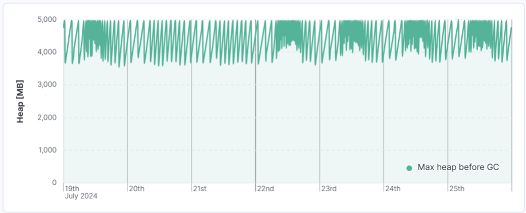
Figure 1. Saw tooth shape of heap utilization. Notice change in pattern during the weekend.
We can utilize the power of aggregations and graph in Kibana two values – a minimum of heap utilization after GC and maximum before GC. This will tell us when GC is starting to collect and how much can it collect. Since Elasticsearch can store huge amount of data we can keep months or even years of GC log history and check if there are any signs of slow memory leak and maybe track when it was introduced to the system.
Here we have an example where a node left the cluster due to long GC pause. This we knew upfront from application watchdog mechanism which terminates the application in such case. But why the long pause? When we saw GC logs from last two months, it became clear that we’re dealing with memory leak. The next question was: when did it start? Was it one of the software versions that introduced it at some point? To answer that we indexed all the history of GC logs we had, and it became clear that it was there from day one. It just didn’t appear due to frequent changes in services and feature deployments in the beginning of the project which required restarts of JVM process. When platform reached its stability the leak weas no longer concealed by frequent restarts. More and more memory was consumed leading to a preventive restart by watchdog process.
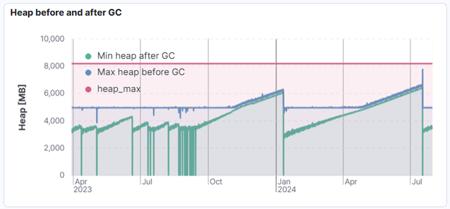
Figure 2. Slow memory leak.
But why hasn’t it restarted in January? Turns out that the deployment which occurred back then, together with the restart of the application, was done in that last possible moment. A day or two later and application would suffer from long pauses and the restart would most probably occur in a following week or two.
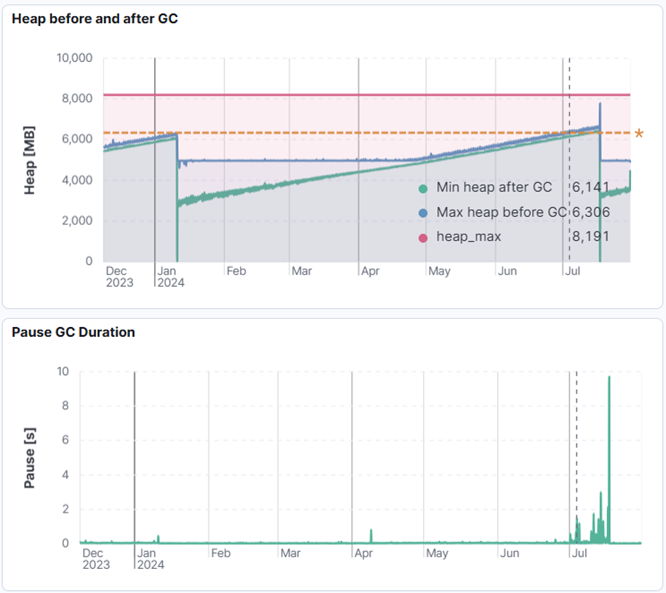
Figure 3. Heap utilization with GC pauses.
Restart in January done in last possible moment before long pauses and restart.
Capacity planning and stress testing
Similar charts can be used to validate whether your environment can withstand increased number of requests. One of possible scenarios is verification of geo-redundancy capacity. Typically, there are two separate data centres running the same set of services. We want to simulate an outage by redirecting whole traffic to only one of them. This way we can verify if one site can process whole traffic.

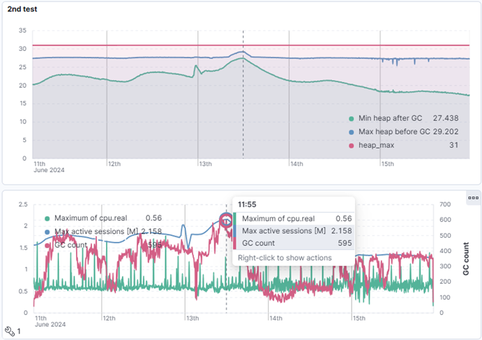
Figure 4 .Two stress tests of a single node.
What you see above is the performance of single node during two such tests. First test ended with node restart due to Full GC which paused JVM for a little over 8s. Graphs on your left-hand side show that it reached just shy of 1.9 million sessions, which was not enough for this test to pass.
Second attempt was made when JVM memory parameters were updated to accommodate increase in the traffic. Current setup passed the stress test reaching above 2.1 million sessions without interruption. As this was enough to conclude the test, we modified load balancer to return to original load distribution. This time we managed to avoid Full GC with long pauses and saved the node from a restart. JVM settings were later propagated to whole environment, so it is now ready for Christmas, New Year’s Eve or any other busy period.
Summary
Garbage collection management is vital for maintaining the stability and performance of modern applications, especially in resource-intensive environments. Analysing GC logs provides valuable insights into CPU and memory utilization patterns, helping teams identify and address potential bottlenecks before they impact users. By leveraging tools like Elasticsearch and Kibana, you can elevate this analysis to the next level. Kibana’s intuitive visualization capabilities enable teams to seamlessly explore GC metrics alongside system events and statistics. This holistic view enables faster root-cause analysis, proactive performance optimization, and smarter decision-making, all of which drive operational excellence and ensure exceptional user experiences.